What Exactly Is a Time Series Database?

Among the many terminologies I’ve heard in the field of databases, time series database is a heavily overloaded concept. Although it sounds simple, its definition becomes quite ambiguous under the packaging of many commercial products. In this article, I aim to provide a clear definition of time series data to help you understand why there is such a category of databases, what scenarios it should be used for, and how to correctly model your data as time series data.
Defining the Time Series Data Model
The data model is a fundamental yet often overlooked concept. We all know that relational databases define relational tables and various operations based on relational algebra, while document-oriented databases treat each piece of data as a semi-structured (JSON) object. Unfortunately, there is no complete consensus on the data model among the time series databases available in the market.
Let’s start with the simplest. A time series is a sequence composed of timestamp-value pairs, usually representing the change of a specific thing over time. Since changes are often continuous, we frequently visualize them using line graphs.

In practice, time series data often appears in groups. For example, if we install monitoring on a server cluster, each node will have a corresponding cpu_usage time series. These time series are all named the same (cpu_usage) and are distinguished from each other using labels (or tags), which are usually in the form of {key=value}.
| Metric Name | Labels | Meaning of Value |
|---|---|---|
cpu_usage |
Cluster name, Node name | CPU usage percentage |
temperature |
Sensor ID, Latitude/Longitude | Current temperature recorded by the sensor |
stock_price |
Stock code | Trading price of a stock |
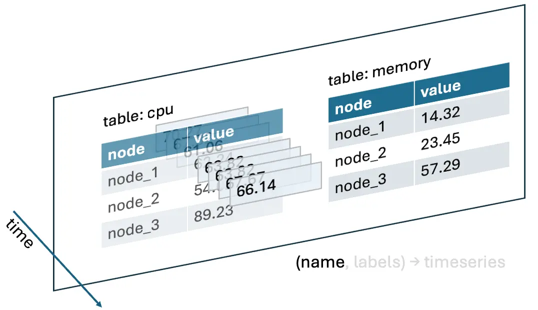
So far, we have three dimensions: timestamp, metric name (or table), and label set, which together uniquely determine a data point (value).
By enumerating all labels into a table, you can draw the following diagram. Here, the XY plane corresponds to the name and labels, and the Z-axis corresponds to time.

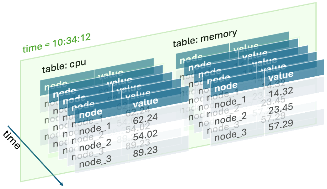
Interestingly, you can view this model from two perspectives:
- : In this perspective, you find a (or a group of) time series vector(s) through the name and labels, and subsequent operations apply to all data points of the current time series. This perspective is closer to traditional relational databases, such as InfluxDB’s InfluxQL, which is designed based on this perspective.

- : In this perspective, you first select a specific time point snapshot, where the values correspond to all time series at this time point. The query language only needs to describe how to process data for a single time slice, as each slice will repeat the exact same calculation. Prometheus’s PromQL is designed this way. 1

Calculation of Time Series Data
With this data model, we can define calculations and queries based on it. Compared to the “2D table” of the relational model, time series data is a set of “3D tables,” with the additional dimension being time. We will see later the special nature brought by the time dimension.
Scalar Operations
Scalar values are calculations on a single value, such as:
cpu_usage * 100converts the CPU usage value from a decimal to a percentage.net_read + net_writesums up the network read and write rates.cpu_usage > 80marks CPU usage greater than 80% as true. 2
Scalar calculations are the most basic calculations, and you can try to understand them from both Perspective 1 and Perspective 2, of course, deriving the same result.
Aggregation
Aggregation in time series databases can be divided into two categories:
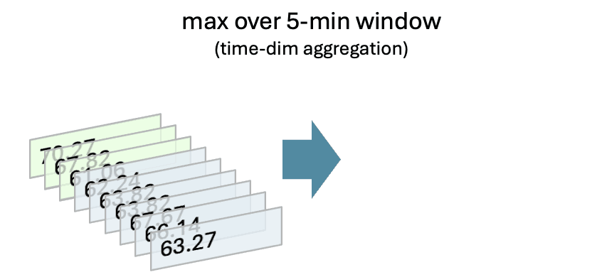
- Aggregation over the time dimension, which applies to each time series, typically includes bucket aggregation, differentiation (growth rate), linear regression, etc., e.g., the maximum CPU usage rate in a 5-minute window.
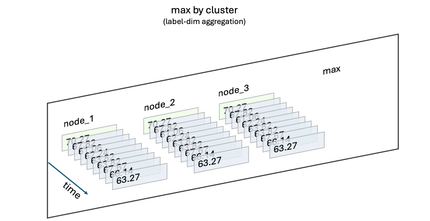
- Aggregation over the label dimension, which applies to each time slice, typically includes sum, quantile, TopK, etc., e.g., the highest CPU usage rate among nodes in a cluster.
Aggregation over the Time Dimension
Taking the most common downsample as an example, it often requires the help of time window functions or the extract() function to align to specific times, such as hourly or daily, and then perform aggregation operations. Since aggregation occurs over the time dimension, it operates on each time series: fn(input: timeseries) -> timeseries.

Particularly, when aggregation over the time dimension encounters a period with missing data points, it often fills with null values or uses linear interpolation between adjacent data points (gap-filling) to make data more regular for subsequent processing. Aggregation over the label dimension obviously does not have this issue.
Aggregation over the Label Dimension
Taking sum (cpu_usage) by (cluster) as an example, it can be understood as performing a group aggregation on cpu_usage for each time slice (Perspective 2):
for each timestamp:
   SELECT cluster, SUM(cpu_usage) FROM cpu_usage GROUP BY cluster

You can also view it as an operation on the entire time series vector (Perspective 1). Implementing it this way is much more efficient than the former, not only because the GROUP BY process is exactly the same each time but also because vectorization can be used to accelerate calculations.
Since multiple time series are usually aggregated, it can be noted as fn(inputs: List[timeseries]) -> timeseries. Since aggregation can be viewed as occurring within each time slice, the time dimension itself (timestamp vector) does not change.
| Aggregation Type | Input | Output | Changes Vector Length | Gap-filling | Example |
|---|---|---|---|---|---|
| Time Dimension | Single timeseries | Single timeseries | Yes | Optional | Maximum CPU usage rate in a 5-minute window |
| Label Dimension | Multiple timeseries | Single timeseries | No | None | Highest CPU usage rate among nodes in a cluster |
Besides the conceptual differences, the two also differ in implementation. Most time series databases have specialized time series vector data structures, using columnar structures to store timestamps and values continuously in files and memory, thus compressing space and improving query speed. Although both can benefit from columnar memory structures, aggregations over time and label dimensions are entirely different operator implementations, which is evident from the input alone: the former inputs a single time series, while the latter inputs multiple time series.
In some SQL-compatible time series databases, both types of aggregation are represented using
GROUP BY, with the actual implementation depending on whether theGROUP BYfield is a timestamp or a label.
Join Operations
Join operations usually occur across both time and label dimensions, aligning two time series vectors by timestamp, where each value corresponds to another value. Note that due to collection delays, the timestamps of each time series may not be perfectly aligned.
Understanding Join operations from Perspective 2 is easier: perform Join operations on a 2D relational table at a specific time slice. The only remaining issue is how to align the two time series to the same time slice. One simple method is to align them at specific intervals, such as rounding timestamps to the nearest minute; another common approach is AS OF JOIN, for example, t1 AS OF JOIN t2 associates t2’s timestamp with the latest and less than t1’s timestamp, expressing the meaning: at the time t1 happens (“as of t1 happens”), what is the value of t2.
Case Study
Prometheus
The data model of Prometheus largely aligns with the definition above. In Prometheus, each metric is a timeseries with a name (metric name) and a set of labels, such as cpu_usage{cluster="prod", node="node1"}.
Prometheus’s query language, PromQL, is designed based on perspective 2, which involves performing operations on values at specific time slices, such as max(usage_usage{cluster="prod"}). The “specific time” is called alongside the query as another parameter. For operations spanning multiple times, such as the rate growth rate = (latest value - oldest value) / elapsed time, PromQL provides the [] operator to extract timeseries from the current query time point back a certain period, such as rate(count_requests[1m]), which calculates request throughput over the past minute.
In actual use, to draw change curves, you often need to query data over a range of time at once. This requires using the Range query API, specifying the start time, end time, and step size, for example:
$ curl 'http://localhost:9090/api/v1/query_range?query=up&start=2015-07-01T20:10:30.781Z&end=2015-07-01T20:11:00.781Z&step=15s'This is fully equivalent to issuing multiple instant queries and then merging the results into a single timeseries.
PromQL’s design is very simple and easy to understand, but it lacks expressiveness in some scenarios. For example, for max_over_time, it had to introduce a complex and inefficient subquery.
InfluxDB
InfluxDB is another popular time-series database, and its data model also aligns with the definition in this article. In InfluxDB, each timeseries has a name (measurement), a set of tags, and fields. Its query language, InfluxQL, mimics SQL syntax and is designed based on perspective 1 or a data-oriented perspective.
InfluxDB’s internal storage engine, Time-Structured Merge Tree (TSM), divides the same table into multiple timeseries vectors based on tags and sorts them by timestamp. Since tags are used to identify different timeseries, you must be careful not to have too many tags, or it will result in too many timeseries vectors, affecting query performance.
GrepTime
GrepTime is an emerging time-series database whose data model aligns with the definition in this article. Each timeseries has a name (metric name) and a set of tags and can contain multiple fields. Since it borrows from the relational model, it is also very similar to InfluxDB.
GrepTime uses an LSM-Tree storage engine, but note that its SST files use a columnar format (Parquet) and are sorted in the order of (tag-1, …, tag-m, timestamp). This likely ensures query performance while balancing update and point query performance.
TDEngine
TDEngine’s data model aligns with the definition in this article. Each table has a name and a set of tags and can contain multiple fields. Since it borrows from the relational model, it is also very similar to InfluxDB.
In its early stages, TDEngine, for efficiency reasons, recommended users create a table for each collection point. However, as scale increased, it became necessary to constantly rewrite queries to reference more tables. Therefore, TDEngine introduced the concept of “super tables,” which divides a logical table into different subtables based on different tags. This design is very similar to InfluxDB’s TSM.
TimescaleDB
TimescaleDB does not conform to the definition of a time-series database in this article. It is more like a relational database optimized for cold data. Considering it is an extension of PostgreSQL, this is not surprising.
This blog post reveals TimescaleDB’s internal storage structure: on top of the original table structure of PostgreSQL, it reorganizes “cooled” data in an array-like format, sacrificing update performance to gain scan performance and compression ratio.
TimescaleDB follows the general relational database model, allowing you to store almost any time-related data in TimescaleDB. Its advantage lies in leveraging PostgreSQL’s powerful features, such as indexing, transactions, foreign keys, etc. However, because it lacks specialized timeseries vector objects, it cannot fully exploit performance advantages when handling standard time-series data (such as metrics).
QuestDB
QuestDB also does not conform to the definition of a time-series database in this article. It is a database optimized for append-mostly workloads, with extremely high ingestion performance. It is based on a simplified relational model, including index, join, etc.
QuestDB uses the simplest and most straightforward columnar storage structure: new data is continuously appended to the latest chunk. However, for updates, it requires more complex versioning and a background Vacuum mechanism, which is why QuestDB is not suitable for scenarios with frequent updates.
Similarly, if your data perfectly fits the definition of time-series data, you should choose a specialized time-series database.
-
The PromQL documentation introduces the Instant vector concept to distinguish between metrics and constants (e.g.,
cpu_usage > 80). But this is merely a difference in terminology. ↩︎ -
In Prometheus’s PromQL,
cpu_usage > 80filters out data points greater than 80% instead of returning a boolean time series. ↩︎